
Gabor-Granger pricing analysis: A working guide for B2B SaaS founders
The most widely cited price-research framework in market research, adapted for software companies with small customer bases and buying committees.
Gabor-Granger is a stated-preference pricing research method that maps a price-demand curve by asking buyers their intent to purchase at multiple price points, then converts that stated intent into expected purchase probability and revenue. The output is the price that maximises expected revenue per prospect, holding product and audience constant.
Three things are worth noting in that definition before going further.
It produces a curve, not a number. A defensible Gabor-Granger output is always a range with named assumptions. Anyone selling you a point estimate is selling you confidence, not analysis.
It maximises revenue, not profit and not lifetime value. Those are different optimisations, with different inputs. The framework cannot tell you how to package, position, or restructure. It only tells you where a fixed offer maximises revenue.

History behind the framework
The method was developed in the 1960s by André Gabor and Clive Granger, two economists at the University of Nottingham. They were trying to solve a pedestrian problem: how do you set the price of a consumer good when there is no existing reference price in the market?
Most of the published material on Gabor-Granger sits in FMCG and consumer-goods research handbooks. Adapting it for B2B SaaS, where sample sizes are smaller, buying decisions involve committees, and renewal behaviour is structurally different from first purchase, requires modifications that the textbook rarely covers. Those modifications are the second half of this article.


The Question Gabor-Granger answers
At what price point does expected revenue per qualified prospect maximise, holding the product offer and target audience constant?
That precision matters because Gabor-Granger is regularly misapplied to questions it cannot answer. It does not give you the profit-maximising price. It does not give you the LTV-maximising price. It does not handle multi-attribute trade-offs. It does not model competitive response. It does not model network effects.
These are not weaknesses. They are the scope conditions of the framework. Inside the scope, Gabor-Granger is the right tool. Outside the scope, reach for something else.
The Two Methods
Most write-ups present Gabor-Granger as a single procedure. There are two, and they generate measurably different results.
Sequential descending. Each respondent is shown the highest price first, then walked down until they accept. Fast and cheap, which is why it became the consumer-research default. But the anchoring contamination is structural: by the time the respondent sees the middle price, they have already seen the high price, and stated willingness to pay drifts upward. For any study where the absolute revenue-maximising number matters, sequential descending overestimates it.
Random monadic. Each respondent is shown exactly one price, randomly assigned. No anchoring because no respondent sees multiple prices. Cleaner data, but the sample requirement multiplies. For five price points and equivalent statistical power, you need roughly five times the sample.
For B2B SaaS, random monadic is the right call when the sample is there. When it is not, the alternative is structured willingness-to-pay interviews, not sequential descending.
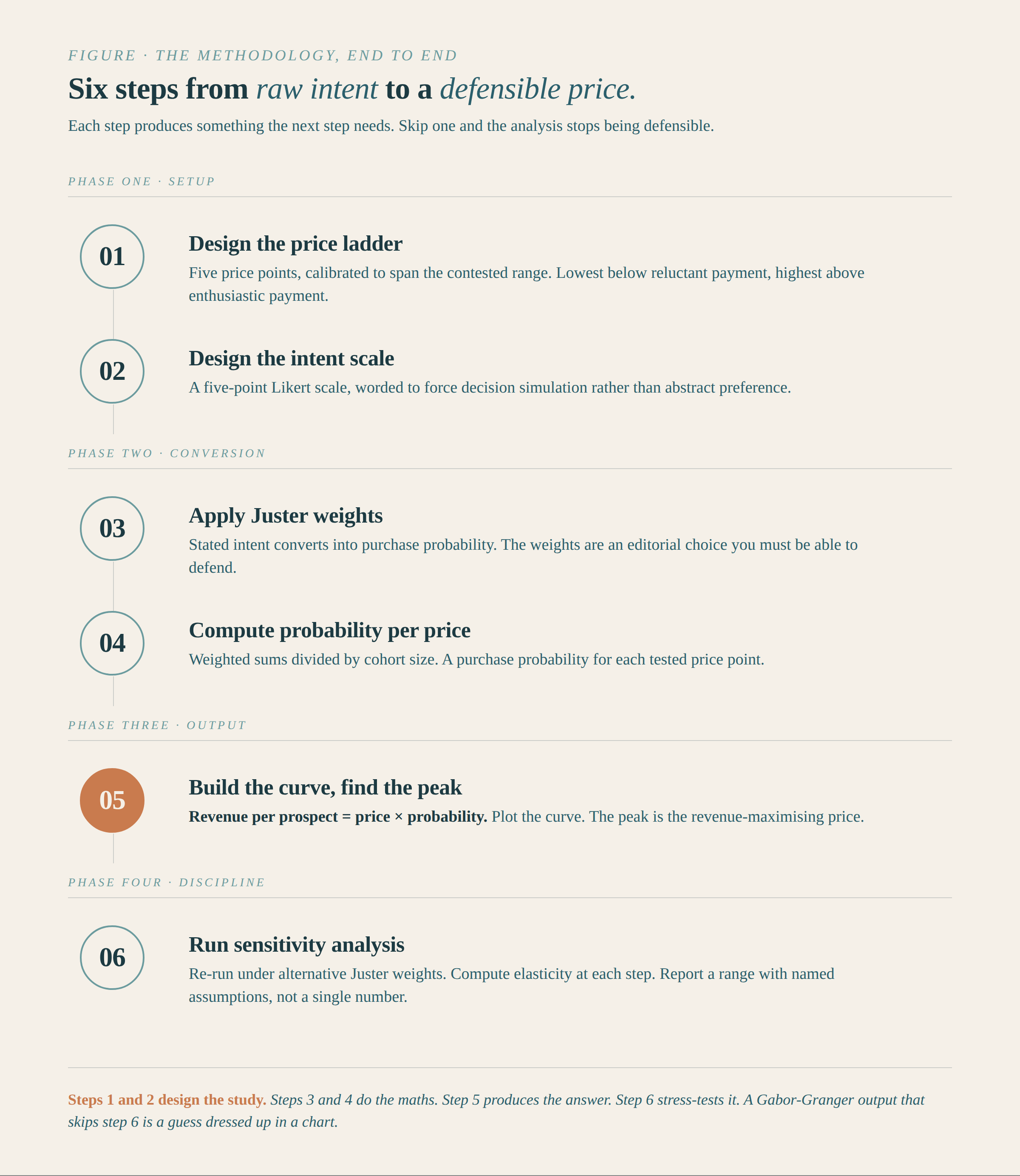
How to run a Gabor-Granger study
Step 1: Design the price ladder
How many points. Five is the sensible default. Three is too few to see curve shape; seven is data-greedy. Five gives you the curve, the peak, and a buffer to verify the shape is plausible.
The range. Too narrow and you cannot see the inflection point. Too wide and the extreme points are wasted data. The lowest point should sit below what any qualified segment would pay reluctantly. The highest should sit above what your most enthusiastic segment would pay comfortably. The middle three test the contested region.
The spacing. Linear spacing (£10, £20, £30, £40, £50) feels natural but treats each pound as equally informative. Logarithmic spacing (£10, £20, £40, £80, £160) is technically more correct: perception of price follows Weber-Fechner, proportional rather than absolute. For B2B SaaS within a tight range, linear is fine. Across an order of magnitude, use logarithmic.
Step 2: Design the intent scale
Respondents answer on a Likert-style scale. The industry standard is five points.
The exact wording matters. "Would you purchase at £X?" generates different responses than "How likely would you be to purchase at £X?" or "If MetricFlow Pro cost £X per month, how likely would you be to buy a subscription?" The third version is the most reliable because it forces the respondent to mentally simulate the actual decision rather than answer abstractly.
Step 3: Convert stated intent to purchase probability
Here is where most write-ups skip the most important step.
Respondents who say they "definitely will buy" follow through perhaps 60-80% of the time, depending on category. Respondents who say "probably will buy" follow through perhaps 20-40% of the time.
The correction applies probability weights to each response. Common weights for B2B SaaS in the £200-£2,000 per month range:
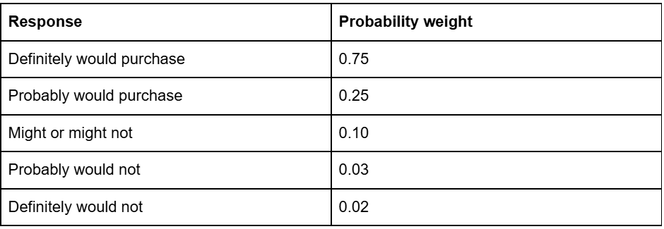
These weights are not universal constants. In FMCG, "definitely" weights closer to 0.85 because the purchase decision is low-stakes and rapid. In enterprise software with six-figure annual contracts, "definitely" weights closer to 0.50 because the buying committee dynamic kills many stated intentions. The B2B SaaS mid-market weights above are defensible for considered purchases at the £200-£2,000 monthly range
The first thing to internalise: these weights are an editorial choice you must be able to defend. That sensitivity range, not the central estimate, is the study's actual output.
Step 4: Compute purchase probability at each price
For each price point, multiply each response count by its probability weight and sum. Divide by total respondents in that cohort. The result is the expected proportion of respondents who will purchase at that price.
Purchase probability at £400 = 10.26 / 40 = 25.7%. Of every 100 qualified prospects shown the product at £400 per month, roughly 26 are expected to actually buy.
Step 5: Build the curve and find the revenue maximum
Repeat the calculation for each price point.
Expected revenue per prospect equals price times purchase probability. The peak of the column is the revenue-maximising price.
Step 6: Run sensitivity analysis
Never communicate a single point estimate. The peak at £300 implies a precision the data does not have. Three sensitivity checks every credible Gabor-Granger analysis should run:
Confidence intervals on each probability.
Reweighting under alternative Juster weights.
Elasticity calculation.
A defensible output looks like:
"Under standard Juster top-two-box weighting, the revenue-maximising price for the Pro tier sits in the £300-£400 per month range, with the curve relatively flat between those points. The peak is sensitive to weight choice: under conservative weighting, it shifts to £250. With CAC of £300 included, the profit-maximising price is likely £400-£500 rather than the revenue maximum."
Adapting Gabor-Granger for B2B SaaS
Small samples need different statistical treatment. For B2B SaaS with 30-150 qualified prospects per cohort, treat each price point's purchase probability as a Bayesian estimate. With small samples, the noise around each point is large enough that the shape of the curve matters more than the exact value at any single point.
Buying committees mean the respondent is not always the buyer. The designer answers enthusiastically; the CFO blocks the renewal six months later. The Juster correction does not handle this because it was developed for individual consumer behaviour. Two mitigations. Screen respondents for actual purchasing authority before including them. Apply a committee-discount factor to "definitely would purchase" responses for products above the typical individual approval threshold (roughly £300-£500 monthly). For mid-market B2B SaaS, 0.7 to 0.8 is a reasonable starting point.
Renewal behaviour differs from acquisition behaviour. A standard Gabor-Granger captures willingness to pay for new purchase. It says nothing about retention at that price. Customers acquired at higher prices often retain better because they self-select into higher-value segments. Layer Gabor-Granger with cohort-retention analysis from existing customer data, segmented by initial price paid.
Network effects move the target. Products that get more valuable with adoption have demand curves that shift over time. The snapshot at T1 differs from T2. For collaboration tools, communication platforms, and marketplaces, Gabor-Granger is a sense-check, not a commitment.
What it costs to get Gabor-Granger wrong
Three failure modes appear more often than the rest.
Treating the output as a number, not a range
The most common mistake. A founder runs a Gabor-Granger, sees "revenue maxes at £20," raises the price to £20 on Monday, and watches churn spike six months later. The curve told them the revenue-maximising price among prospects considering purchase today. It said nothing about existing customers facing a renewal decision, who behave very differently.
The fix is not better methodology. Existing-customer pricing is a separate question, usually answered with a different methodology.
Using sequential descending without acknowledging the anchoring effect
Many published Gabor-Granger studies, particularly older ones in FMCG, use the sequential descending version without flagging the anchoring contamination. Their revenue-maximising prices are systematically too high. If you read such a study to benchmark your own pricing, you will price too aggressively.
Ignoring competitive substitution
Gabor-Granger assumes the respondent's purchase decision is between "your product at price X" and "no product." For categories with weak competitive pressure, that is approximately true. For categories with strong substitutes (most B2B SaaS), it is not. The respondent who declines your product at £20 may be buying a £15 competitor, not staying out of the category.
The fix is to include competitive context in the survey design. Either ask the price question alongside a named comparator ("Product X costs £15 for similar functionality. At £20 for your product, how likely would you be to buy?") or run the survey on a sample of buyers who are not currently using a competitor.
If you are running pricing analysis on your own SaaS business and want a second pair of eyes on the methodology, the Revenue Architecture Audit is a structured way to pressure-test your pricing decisions before they become contract terms. Details at nirgrowth.com.
NIR Growth helps B2B SaaS founders at £1-10M ARR build the pricing architecture for their next stage of growth. Gabor-Granger, Van Westendorp, conjoint, and the diagnostic frameworks that sit underneath them.